Draper INternship:

I worked as an intern at the Draper Laboratory in the summer of 2019.

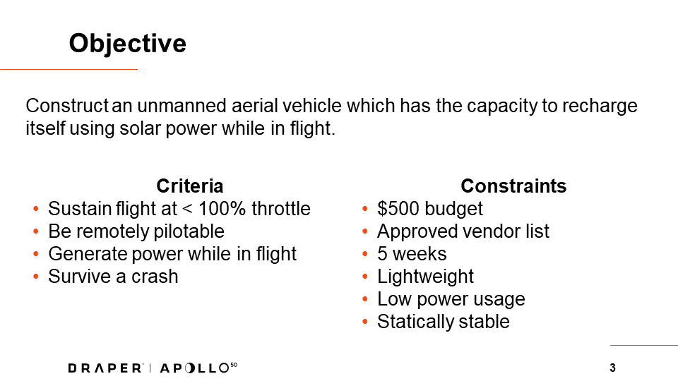
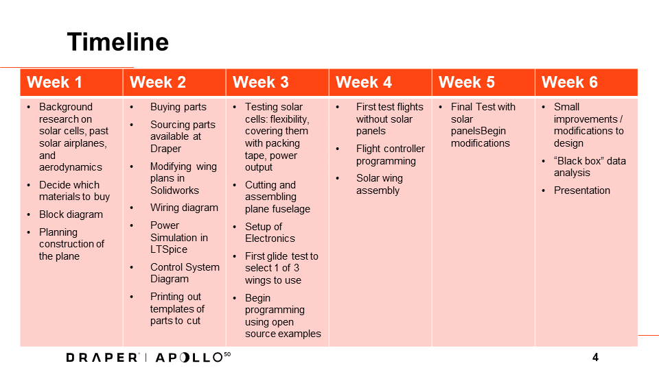
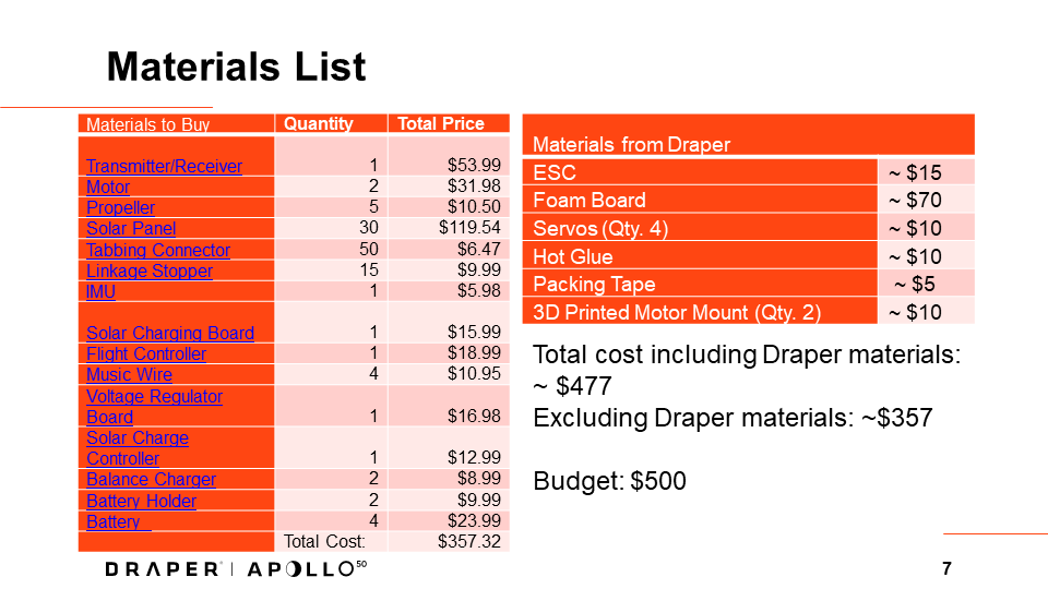
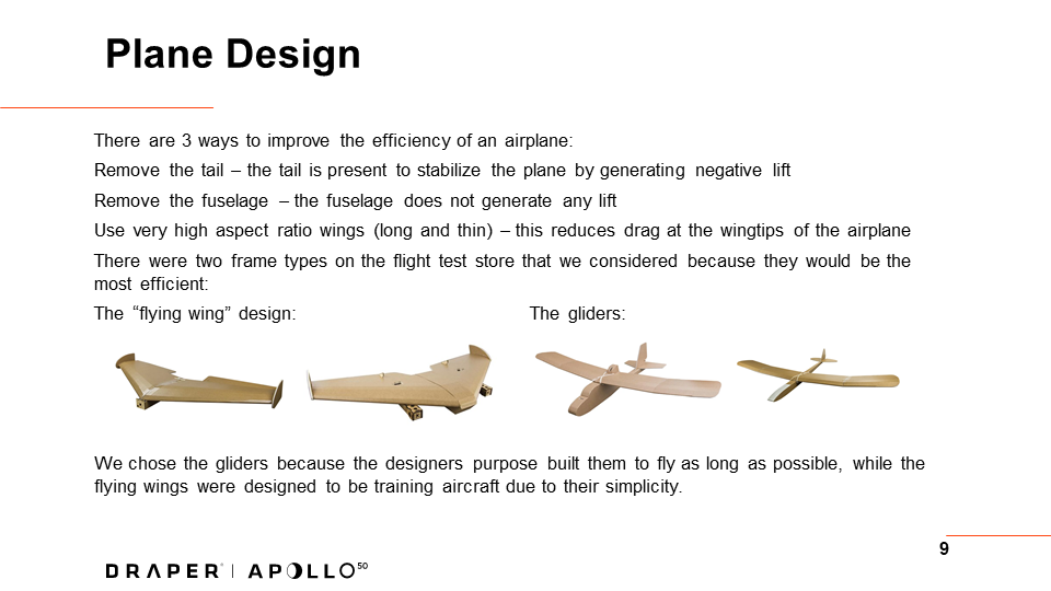
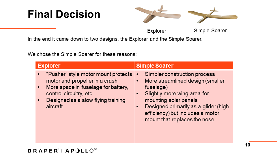
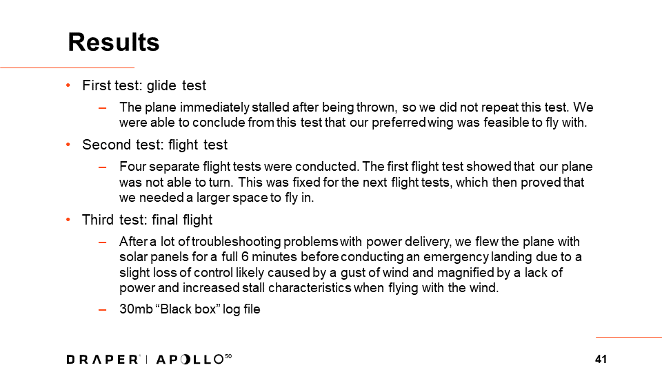
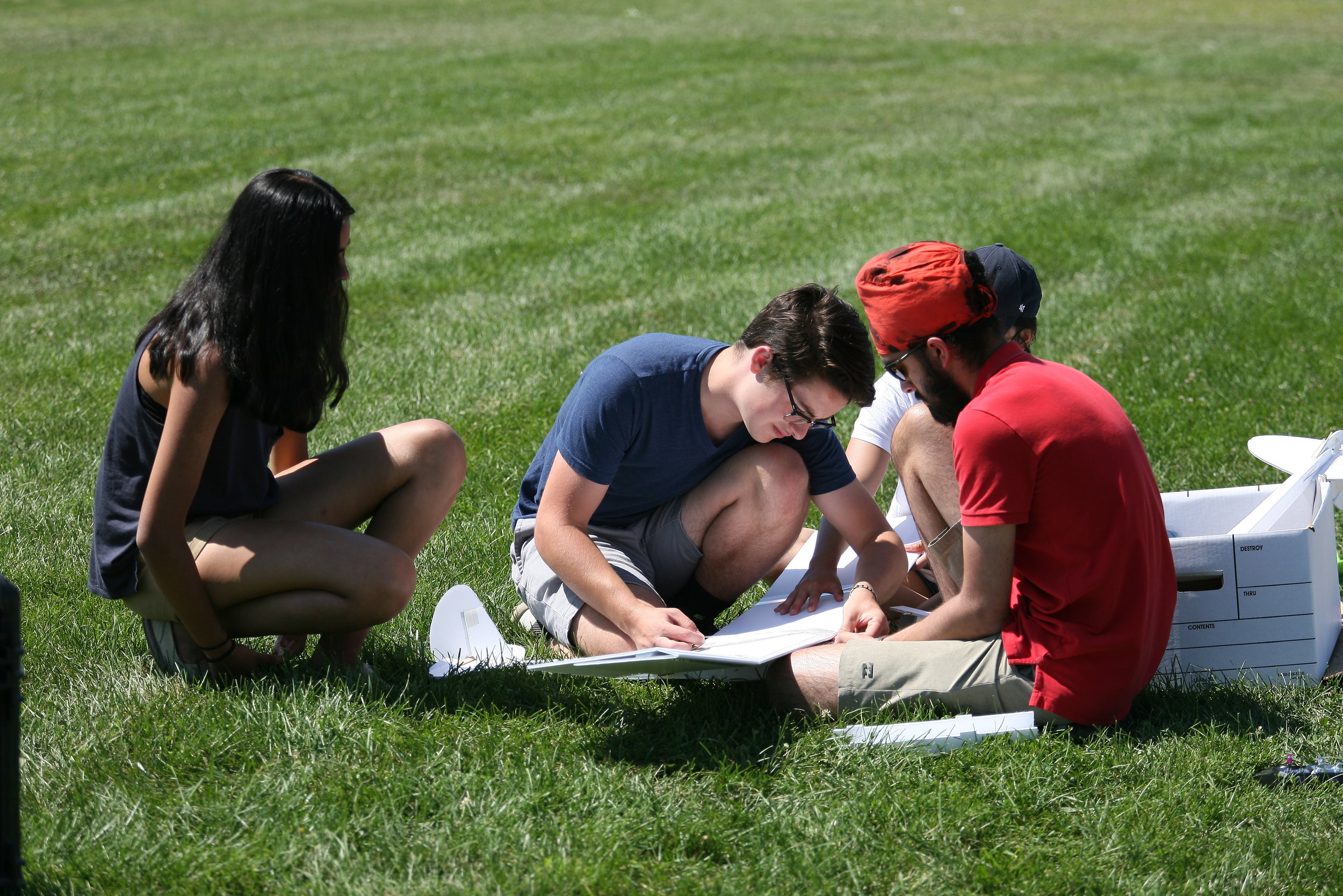
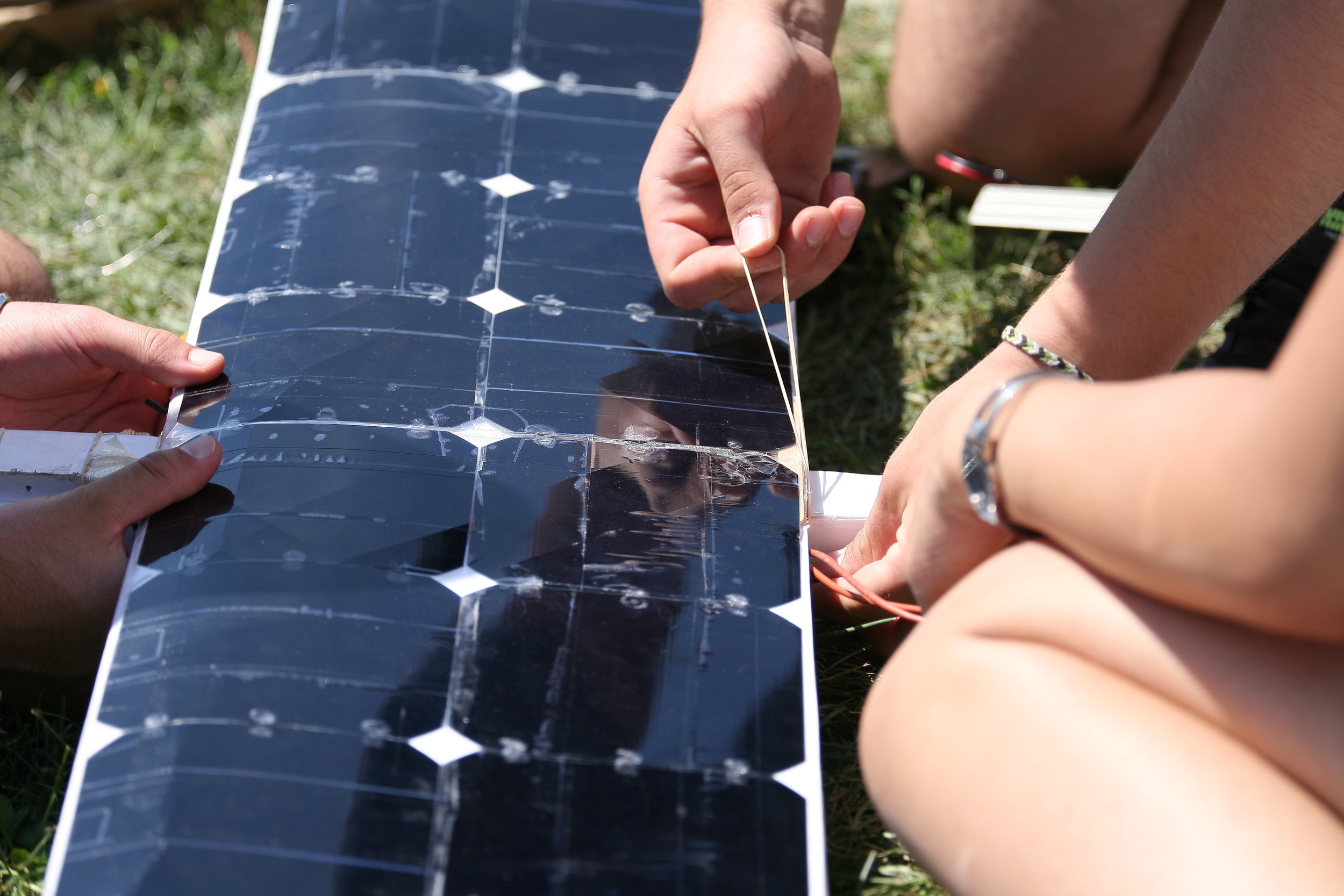
I, along with 3 other highschoolers, was tasked with building a solar powered plane. We had 6 weeks and $500 to work with, along with the various tools and basic materials already available at the laboratory. Throughout the course of the internship, we ran power simulations, soldered together and programmed a flight controller, tested the solar panels, built the aircraft and performed test flights. Our final result was a 6 minute flight which was cut short due to turbulent winds, but the solar panels did generate energy and charge the plane’s batteries.

Presentation:

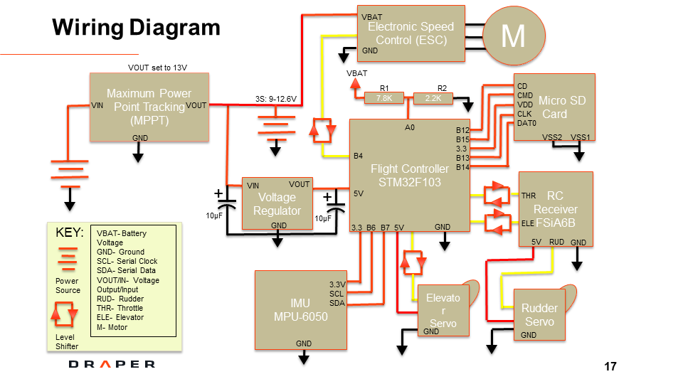
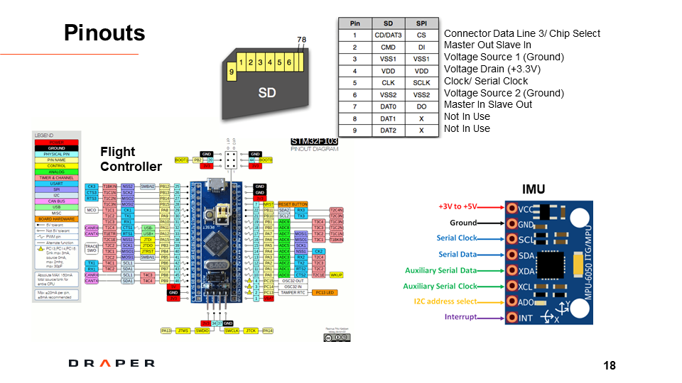
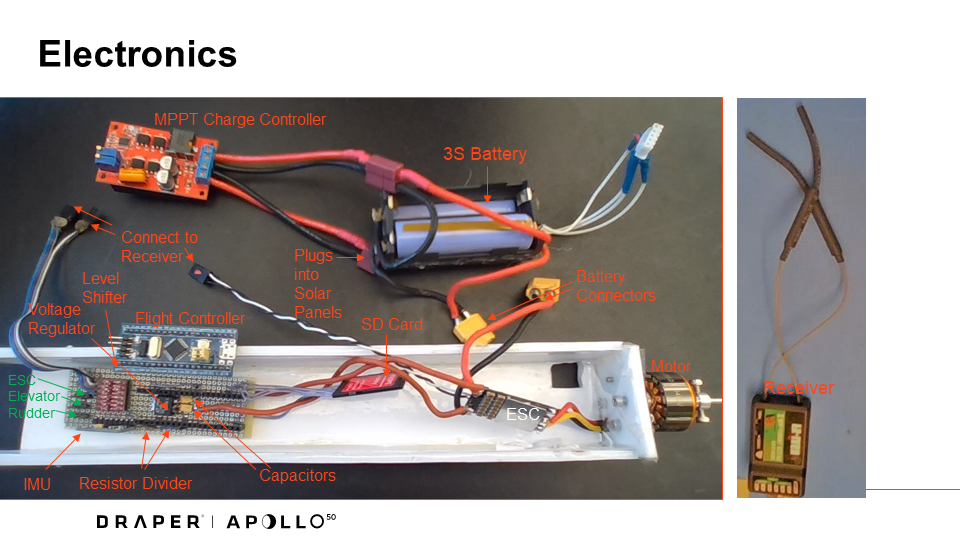
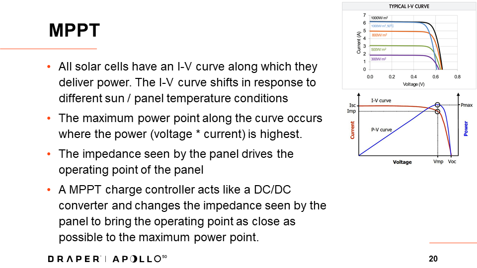
Here is the final presentation we gave at the end of our internship. It is very in depth, so feel free to skim it. The parts I worked on specifically were the electronics, solar panels, power simulation, and data analysis.

Gallery:

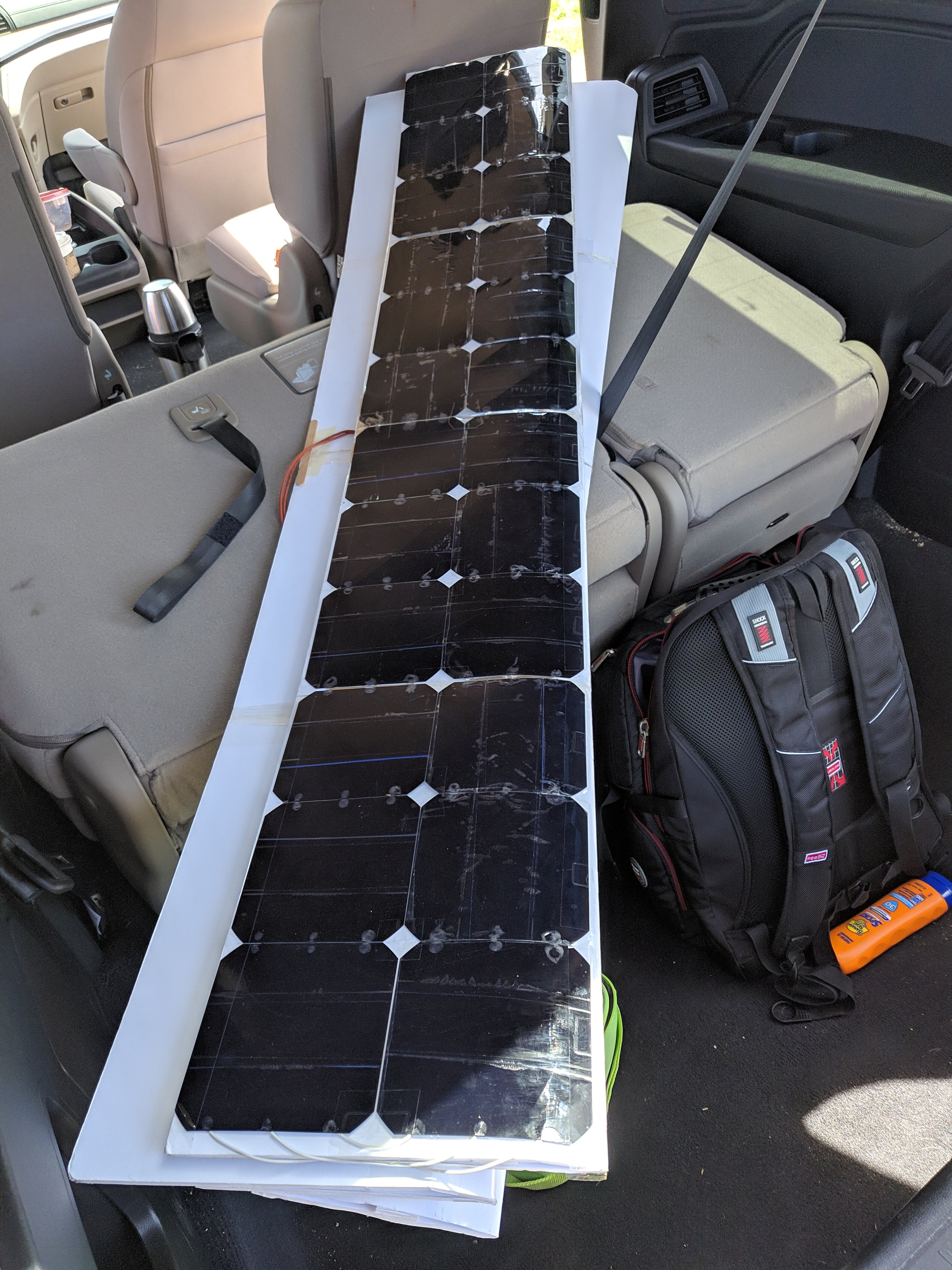
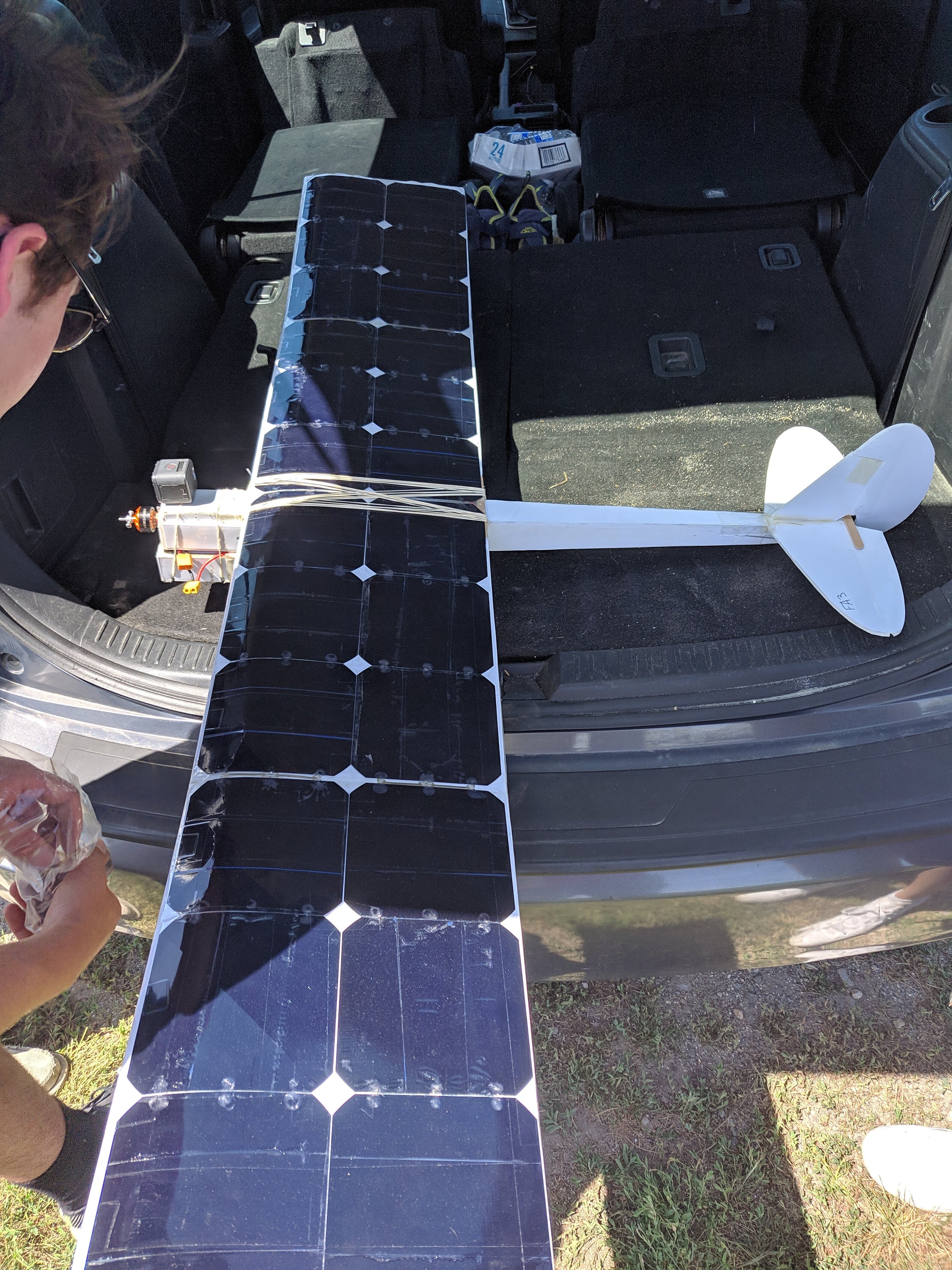
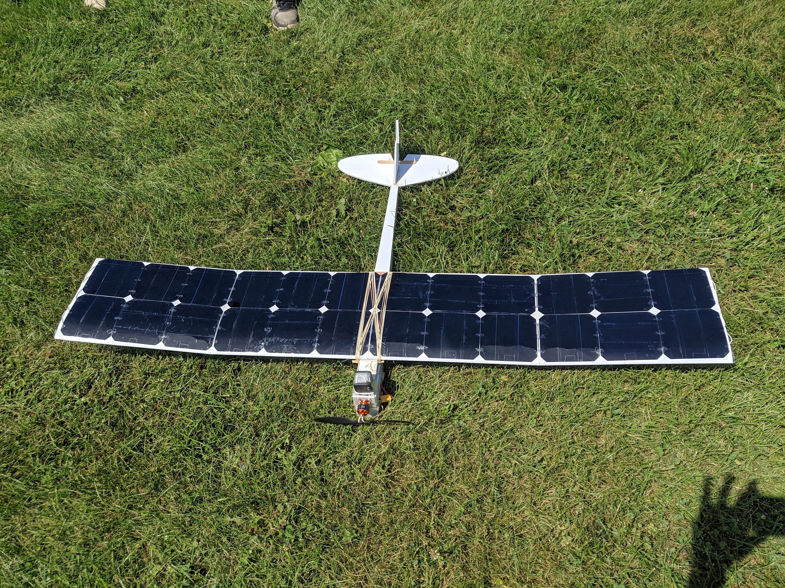
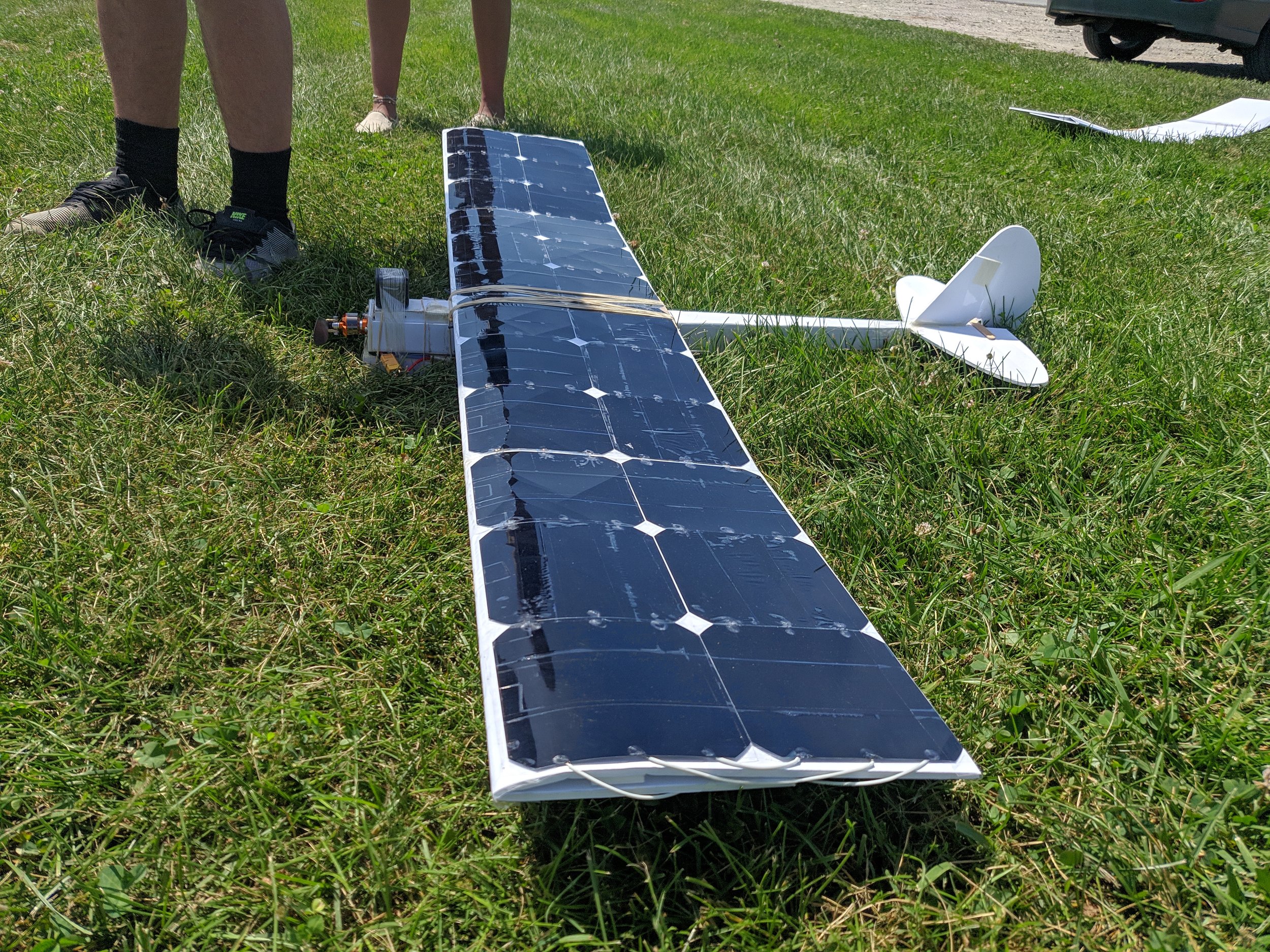
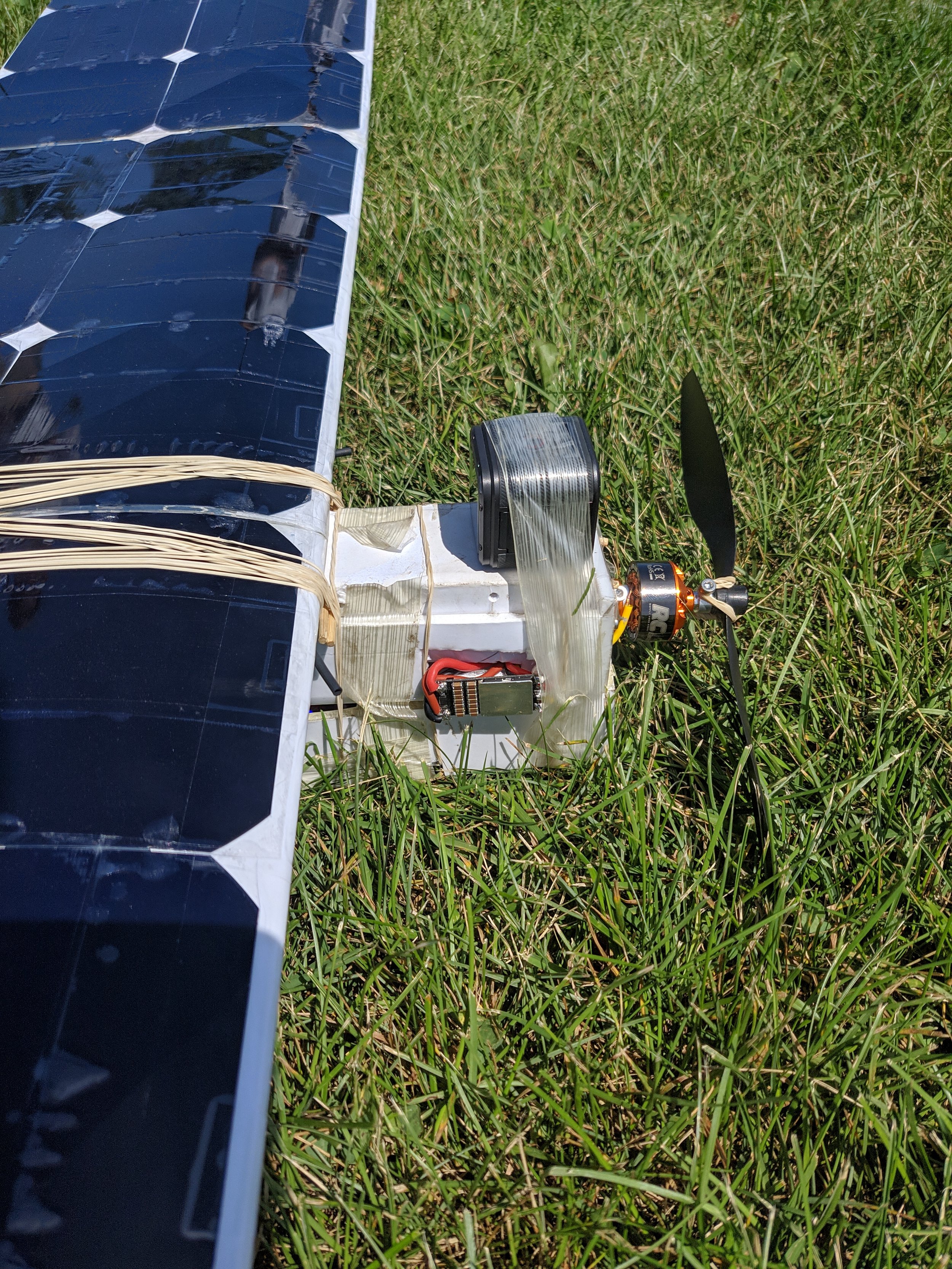
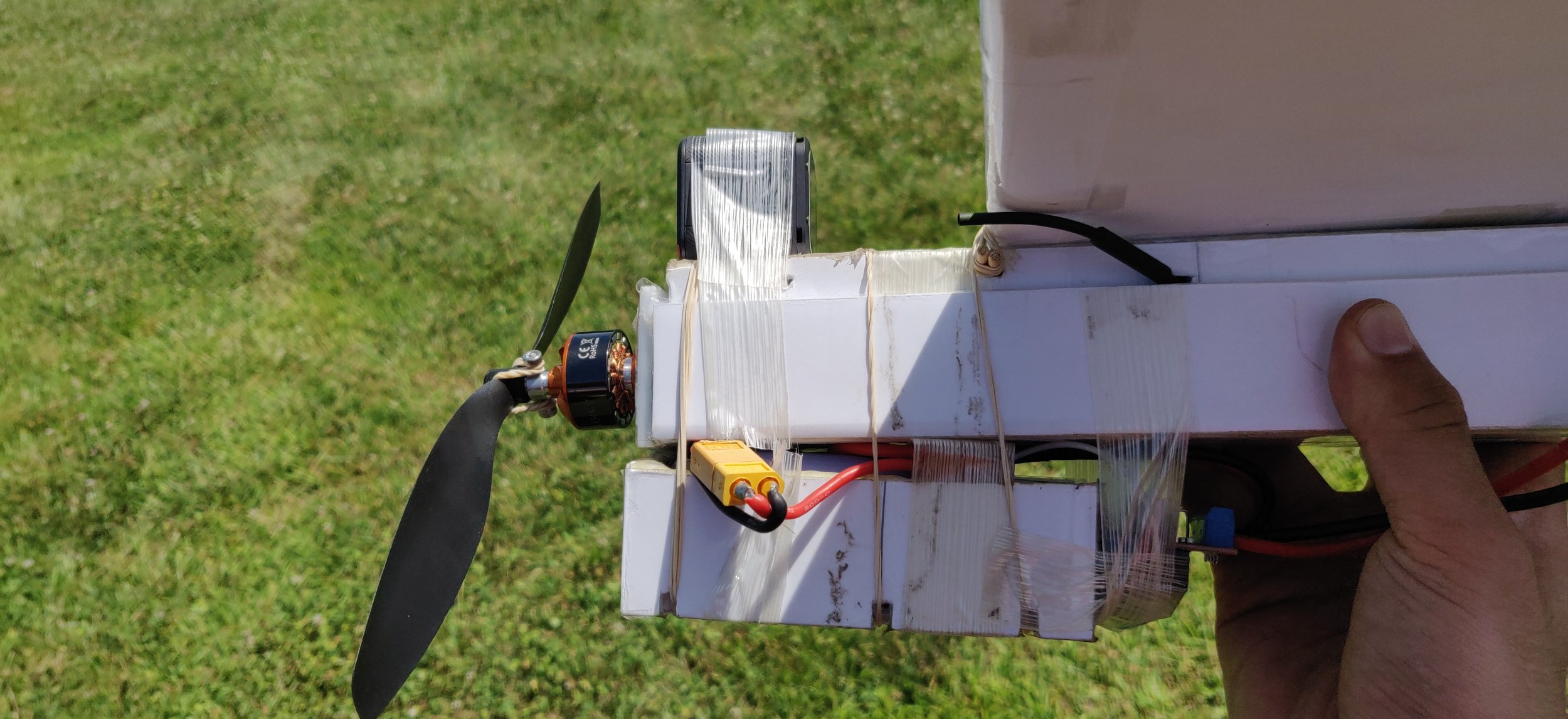
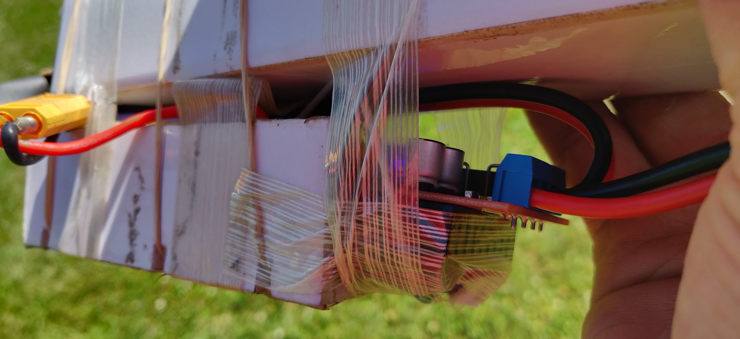
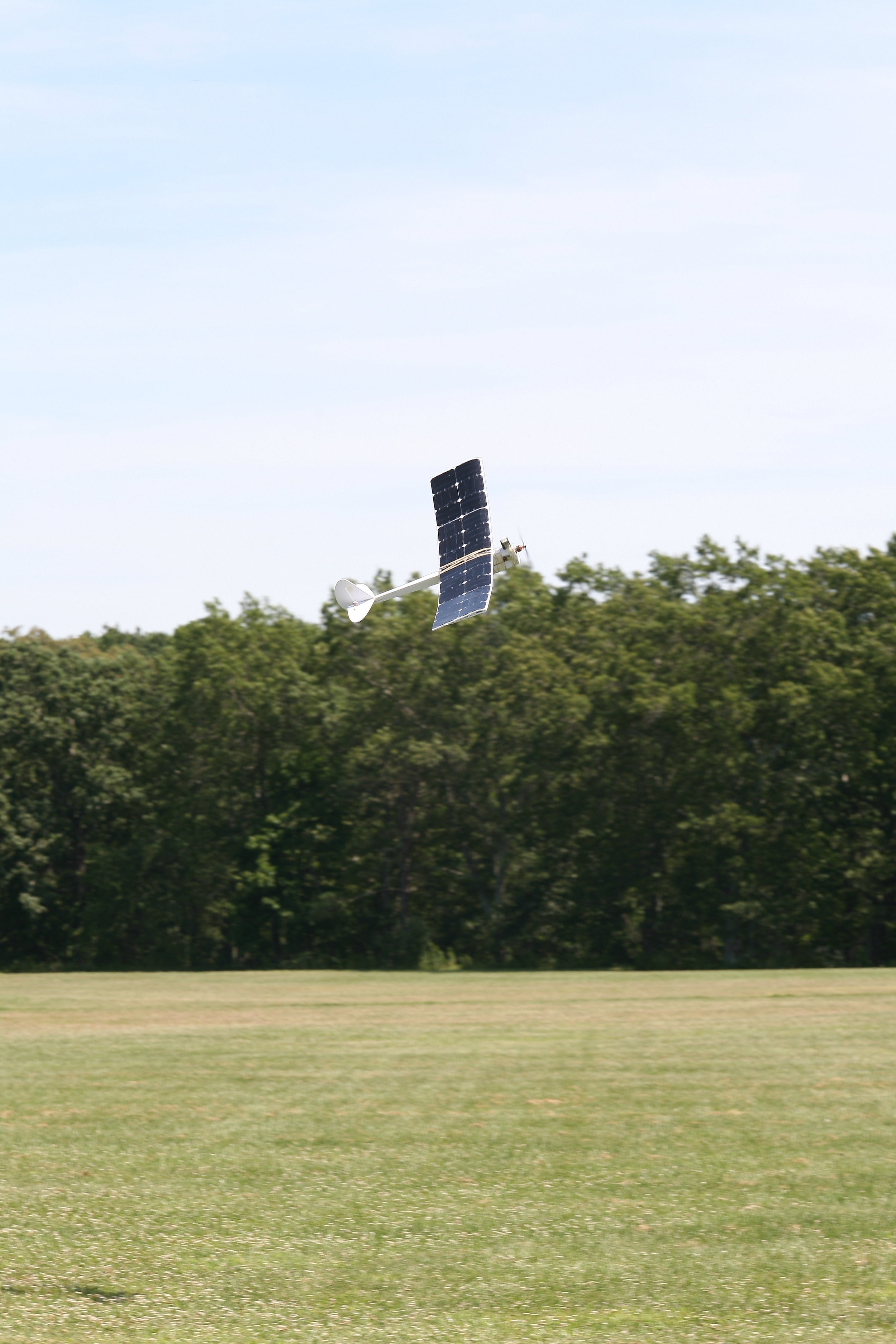
These pictures were taken on the day of the final test flight which was the only one to use the solar wing. In the side views of the plane, the battery pack is visible held on to the bottom of the fuselage using rubber bands. This was done because the fuselage lacked space for the batteries and solar charge controller. Also, since the nose would contact the ground first in a crash, the battery pack would detach reducing the impact felt by the fuselage. For this reason the wings are also attached using rubber bands instead of a hard mount.

Gopro footage:

This is the video from the backwards facing GoPro camera mounted on the front of the plane. The plane is very unstable in the roll direction because there are no ailerons on the wing. The only control surfaces of the plane are on the tail (rudder and elevator) for pitch and yaw to maximize the available wing area for solar panels. The wings do have a dihedral curve to improve stability but it can only help so much without active control.

Data Analysis:

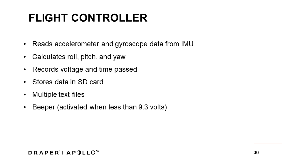
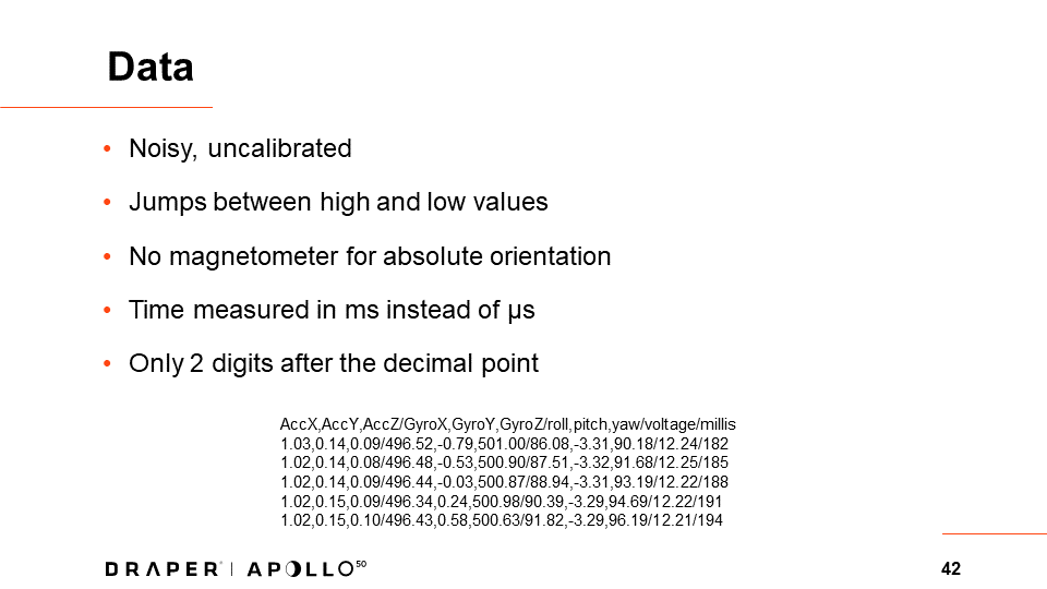
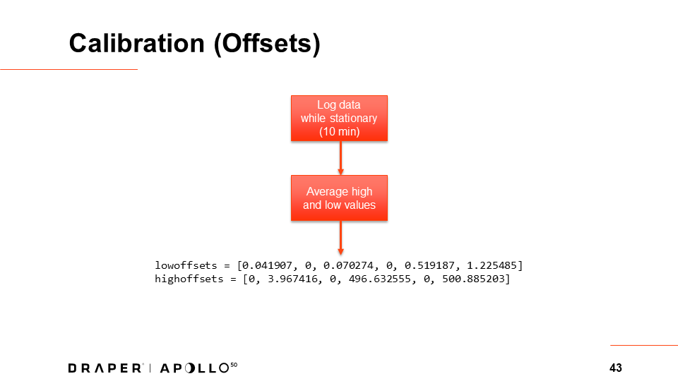
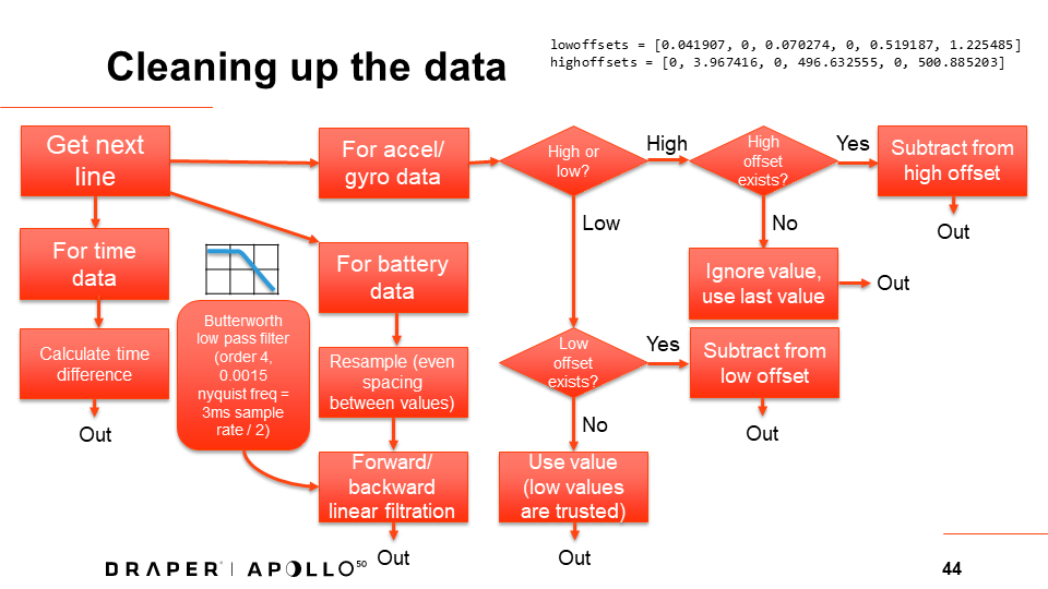
Throughout the 6 minute flight, the onboard microcontroller recorded the battery voltage, accelerometer and gyroscope data to an sd card every 3 ms. After the flight, the data was recovered, analyzed and visualized using python, numpy, scipy and matplotlib. Unfortunately the raw data was quite messy, with the accelerometer readings randomly jumping up to 4 Gs and the gyroscope readings reaching 500 degrees/sec for no reason (slide 42). To counteract this, the data was first cleaned up by subtracting offsets for each sensor value and butterworth low pass filtering the battery voltage data (slides 43 and 44).

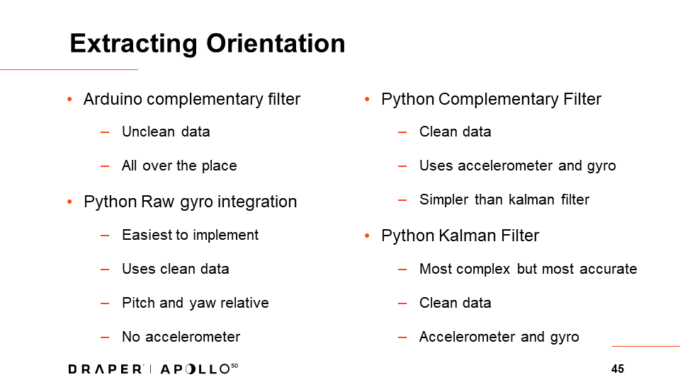
With the clean data, the orientation measured by the sensor was extracted in python using 3 different methods, varying in complexity and accuracy. The fourth method of calculating orientation was done in real time on the flight controller, but was much less accurate due to the fact it was using unclean data (slide 45).

This is a recording of the data visualization for the 6 minute flight. The graph on the left is the battery voltage over time. Blue is the raw data from the SD card and red is the data after it has been low pass filtered. The green line indicates where in the flight the data visualization is at.

The vector graph on the right shows the orientations returned by each of these methods in different colors. For each orientation, the acceleration measurements in x, y and z are rotated in accordance to the returned pitch, yaw and roll values. The least vector on the graph in pink is the total acceleration vector rotated using the kalman filter angles. This acceleration is integrated to get the velocity and vertical velocity shown in the bottom left corner, and double integrated to get the altitude. Since these values are integrated from sub optimal data, they are inaccurate. The playback has been sped up.